
The Star Schema
Facts tables and Measures
A Fact table holds rows of data containing the measures/numbers you wish to analyse. For example, a Sales fact table contains one row per invoice line item with sale amounts, discounts and other measures. A Fact table usually represents a business process or an event in a business process that you want to analyse. Fact tables are often defined by their grain. The grain of a fact table represents the most atomic level by which the facts may be analysed. In this case, the grain of a Sales fact table is individual invoice line items.
Dimensions and Attributes
A standard Dimension defines an entity in a business (e.g. Product, Customer etc), and groups the attributes of that entity together. A Dimension holds the attributes (i.e. fields) you want to analyse your facts by. E.g. Product Type, Product Colour etc. The attributes are used to constrain and group fact data when performing data warehousing queries. E.g. Select Sales Amounts, where Product Colour = Silver. Other dimensions like Time and Calendar are common. We will discuss Dimensions in detail in the Dimension Concepts topic.
Star Schema
A Star Schema refers to the way Facts and Dimensions are related in a Data Warehouse. A Star Schema is organized around a central fact table that is joined to its dimension tables using foreign keys. The name star schema comes from the pattern formed by the entities and relationships when they are represented as an entity-relationship diagram. The fact table of a specific business activity (i.e. the Fact) is at the centre of the star schema and is surrounded by dimensional tables with data on the people, places, and things that come together to perform the business activity. These dimensional tables are the points of the star.
An example:
Suppose a company sells products to customers. Every sale is a business event that happens within the company and the Sales fact table is used to record these events. The Star schema would look like the diagram below.
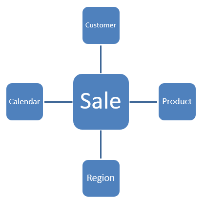
Fact table: Sales
The fact table will contain the measures of the business event (in this case Units Sold and Total Amount) and the foreign keys back to the associated Dimension members. The grain of this fact is one row per sale line item.
| Sale_sKey | Calendar_sKey | Product_sKey | Customer_sKey | Region_sKey | Units Sold | Line Item Amount |
| 1 | 20130321 | 17 | 2 | 1234 | 1 | $ 500.00 |
| 2 | 20130406 | 21 | 3 | 1246 | 2 | $ 345.87 |
| 2 | 20130406 | 17 | 3 | 1246 | 1 | $ 12378.98 |
Dimension table: Customers
The Customer dimension contains 1 row per customer. Each row contains the attributes of that customer. Note that the values for the attributes are verbose descriptions, rather than codes (e.g. Male instead of say 1 for Male). The reason is that these values become column headings in a report, and a column heading of 1 is not very informative. This demonstrates one of the key differences between modelling for a data warehouse and an operational system. A data warehouse contains much data redundancy. It doesn’t follow the conventional ideas of 3rd normal form (3NF) modelling. It like this on purpose. A star schema is a simplified model with easy relationship navigation for end users. That is often a hurdle that DBAs and application developers, coming from a traditional database background, need to overcome, before they can fully embrace Dimensional modelling concepts.
| Customer_sKey | Customer_ID | Full Name | Gender | Club Member | Marital Status | Occupation |
| 1 | 1 | Brian Edge | Male | Is Club Member | Married | Fire Fighter |
| 2 | 2 | Fred Smith | Male | Is Not Club Member | Single | Police Man |
| 3 | 3 | Sally Jones | Female | Is Club Member | Married | Lawyer |
The fact table contains business events that happen in our company. The dimension tables contain the factors (Customer, Time, Product) by which we want to analyse the facts.
By following the links we can see that, for example, the 2nd row in the fact table records the Sales event that customer 3 (Sally Jones) bought two Products (sKey 21 and 17) in Region sKey 1246 on the day corresponding with the Calendar Dimension member with the sKey 20130406. The Product, Region and Calendar sKeys point back to a row (aka a Dimension Member) in their respective Dimensions.
Given this fact table and these three-dimension tables, we can ask questions like: How many (sum of units), diamond rings (product dimension) have we sold to unmarried male customers (customer dimension) in the south region (region dimension) during the first quarter of 2008 (calendar dimension)?
Simply put, organizing data into a star schema like this provides a very simple to understand filtering and aggregation engine. The dimensions are used to filter the set of fact rows that are returned in a query. Aggregation (i.e. SUM, AVG, MAX, MIN etc or more complicated calculation) is applied to one or more of the measures across the rows in the filtered result set. This is a key point. It’s key to understanding how a star schema works, and why it’s a great way to present data for analysis purposes.
Another Star Schema Example
Included with the course is a Data Warehouse Database. This is a database generated by Dimodelo Data Warehouse Studio. There is a fact table called fact_TimeRecord. An excerpt of its star schema diagram for fact_TimeRecord is below.
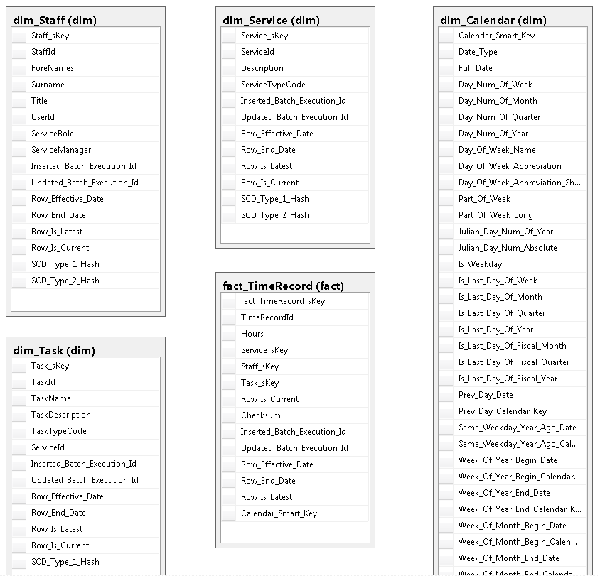
You will notice that there are no relationships shown. This is because Dimodelo Data Warehouse Studio generates Dimensions as ColumnStore indexes by default, and there are no Primary Keys defined. Generally speaking Primary Keys and Clustered indexes will slow down your ETL Load. Most queries for reporting should occur against your OLAP Cube, so not having indexes will not impact report generation time. In any case, a ColumnStore will perform much better for aggregated queries over random attributes (that you see in reports) than clustered indexes.
Try this query against the star schema:
SELECT c.Year_Num, s.ServiceTypeCode, St.ServiceRole, SUM(Hours) AS Sum_Hours
FROM fact.fact_TimeRecord f
JOIN dim.dim_Calendar c
ON c.Calendar_Smart_Key = f.Calendar_Smart_Key
AND c.Year_Num = 2015
JOIN dim.dim_Service s
ON s.Service_sKey = f.Service_sKey
AND s.ServiceTypeCode = 45
JOIN dim.dim_Staff st
ON st.Staff_sKey = f.Staff_sKey
GROUP BY c.Year_Num, s.ServiceTypeCode, St.ServiceRole
It returns this result:
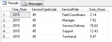
The Sum of Hours for the Year 2015 and ServiceTypeCode 45 broken down by Service Role.
Notice that query is simple (although a little long) and the join paths are straight forward. I.e. You are not joining through multiple tables to get an attribute value. This is the simplicity of a star schema model. Filtering using dimension attributes with simple joins to facts and aggregating measures.
One of the advantages of using a Semantic OLAP/Tabular Layer is that it (conceptually at least) writes these queries for you. It’s a drag and drop interface, where you drag the dimension attribute filters, row labels, and column headings onto a pivot table/chart.