Dimension Concepts

Dimensions and Attributes

Dimensions provide the “who, what, where, when, why, and how” context of a business process event. Dimension tables contain the descriptive attributes used by BI applications for filtering and grouping the facts. A standard Dimension defines an entity in a business (e.g. Product, Customer etc), and groups the attributes of that entity together. A Dimension holds the attributes (i.e. fields) you want to analyse your facts by. E.g. Product Type, Product Colour etc. The attributes are used to constrain and group fact data when performing data warehousing queries. E.g. Select Sales Amounts , where Product Colour = Silver.

Definitions

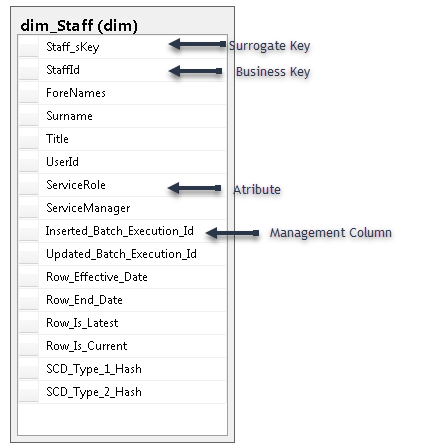
• A Dimension contains Members. There is a Member for every business/natural key of the dimension. However, because a Dimension can keep a history of change, there may be multiple versions of a Dimension member. This mean that the business/natural key might be duplicated. Therefore each version of the dimension member is assigned a unique surrogate key by the data warehouse. Usually a surrogate key is an integer sequentially assigned. There are cases where you may want to use a “smart” key, or code for the surrogate key. A typical example is the Calendar Dimension, with a smart key like “YYYYMMDD” is used as the surrogate key for each row (representing a day) in the Calendar. The surrogate key is the primary key of the dimension.
• Attributes. Attributes are the descriptive information for each member. E.g. Product Type, Product Colour etc. Attribute values become row and column headers in pivot tables/charts, so attributes generally contain descriptive data. Operational codes (e.g. 1 for Male, 2 for Female) are generally stored in the attribute with their descriptive format (i.e. as Male/Female). Cryptic abbreviations, true/false flags, and operational indicators should be supplemented in dimension tables with full text words that have meaning when independently viewed.
• Management Columns. A Dimension will also contain a set of “management” columns. Management columns are generally used by the ETL to help load data into the Dimension, and to set properties of each row like latest flag, effective dates etc.

Denormalization

Dimensions tend to be de-normalized. For example, take a Sales Area->Region->State->Country hierarchy, which, in an operational system, would normally be modeled as separate tables. In a dimensional model there would be a single Sales Area Dimension, with attributes for Region, State and Country. The exception would be if there were Facts in the Data Warehouse which had a grain at the State or Country levels, then, it’s necessary to have separate Dimensions for those levels, so those Facts can be attached at that level.

Slowly Changing Dimensions

Dimensions are often referred to as ‘Slowly Changing Dimensions’. This describes the fact that dimensions members are relatively static but do change, albeit slowly, over time. How this change is managed in the data warehouse usually falls into 4 types. Type 1, Type 2, Type 3 and Type 6 (which is a hybrid of type 1 + 2 + 3). The most common are type 1 and type 2. In-fact, I’ve never seen a use case for Type 3. Different attributes within the one dimension can have different slowly changing dimension types.

Slowly Changing Dimension Type 1 – Overwrite

When the Slowly changing dimension (SCD) type 1 is applied, if a change occurs to an attribute, the existing dimension member row is overwritten with the new value of the attribute. Essentially no history is kept. A good example of a Type 1 Attribute is Employee Name. If an employee name changes due to marriage, the Name should be overwritten. This has the effect of moving all history to the Employee’s new name. This highlights unanticipated consequences with type 1. Let’s say you have a Sales Division org unit dimension, and each Sales Division has a parent Region attribute. If the Sales Division moves to a new Region, and the Region attribute of the Sales Division is treated as type 1, then all the historical sales facts that were associated with the original version would suddenly appear in Regional reports as if they belong to the new Region, usually, an undesirable outcome. This is where Type 2 comes in.

Slowly Changing Dimension Type 2 – Add a new Version

In the SCD type 2 scenario, a new version of the Dimension member row is written when a Type 2 Attribute changes. History is preserved. Existing facts remain associated with the old version of the dimension member and new data is associated with the new version of the dimension member. Let’s say you have a Sales Division org unit dimension, and each Sales Division has a parent Region attribute. If the Sales Division moves to a new Region, and the Region attribute of the Sales Division is treated as type 2, then a new row is written to the dimension for the new version of the dimension member. All the existing sales facts that were associated with the old version would still appear in Regional reports as if they belong to the old Region, which is desirable, because this region was responsible for the sales at the time it was made. Only new facts that are associated with the Sales Division after the change will be associated with the new Region.

Hierarchies

• Natural Hierarchies. Many dimensions contain natural hierarchies of attributes. In our previous example, in the Sales Area Dimension there is a hierarchy from Country->State->Region->Sales Area. It’s important that each attribute value belongs to only one of its parent Attribute values. Otherwise you have a broken Hierarchy. Hierarchies can be very useful for analysis, allowing drill-down and drill-up analysis in BI tools. Some Dimensions can have multiple hierarchies. For example, a Calendar Dimension can have a Day>Month>Year… a Day>Month>Fiscal Year… a Day>Month>Quarter>Year and a Day>Fortnight>Year hierarchies. All are valid Hierarchies, and all may be used by different people for different purposes. Hierarchies in a Dimension always end with the root Attribute at the Grain of the Dimension. E.g. In the Calendar Dimension, the Day Attribute.
• Parent-Child Hierarchies. A Parent-Child Hierarchy is a hierarchy of the the same object type. Good example are Hierarchies of Employees or Positions in an Organisation Chart. Each object points to its parent object. Each Position in a Organisation Chart, points to it’s parent Position. A Parent can have multiple children, but a child only has one parent. Parent-Child Hierarchies are also know as Ragged Hierarchies, because each “branch” of the “tree” can have a different number of levels.

 Role Play Dimension

A Fact can be associated with a Dimension more than once in a different role. These secondary associations are known as Role Play Dimensions. For example, the Task fact can be associated to the Calendar Dimension a number of times, once for a Scheduled date, once for a Started date, once for a Completed date and so on. Each of these would appear as separate Dimensions, i.e the Started Calendar Dimension, the Scheduled Calendar Dimension and the Completed Calendar Dimension. This structure allows you to use the Scheduled Calendar, for example, to get the count of Tasks scheduled to start in a month. You could use both the Schedule and Started Calendars to get a count of Tasks that were both Scheduled and Started in a month. If you are querying you relational Data Warehouse directly, it’s useful to create a view for each role play of the calendar. If you are using OLAP, its not necessary.

Junk Dimensions

Transactions typically produce a set of miscellaneous, low-cardinality flags and indicators. E.g. Sale Type, Sale Status etc. Rather than making separate dimensions for each flag, you combine them in a single junk dimension. This dimension does not need to be (but can be) the Cartesian product of all the attributes’ possible values, but should contain the combination of values that actually occur in the source data. The more attributes you have in the Dimension the bigger it gets. Its important that they are low-cardinality. If you have 10 * 345 * 81 * 3 * 21 attribute values you have 17M+ members. So you need to be careful what you include. The business key is the combination of all attributes. Despite this a Junk Dimension is a valuable modelling technique in certain circumstances.

Snowflaked Dimensions

When hierarchical relationships in a Dimension table are normalized, secondary Dimension tables are created and connected to a base Dimension by an attribute key. My advice is to avoid them. They simply make the Data Warehouse harder to navigate, and there is nothing that is modeled in a Snowflake Dimension, that can’t be modeled in a Star Schema.

Many to Many Relationships

Many to Many relationships are defined in a Dimensional model using a Group and a Bridge. Take the example below:

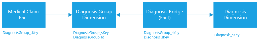
In this example, an insurance company receives medical claims. The medical claims are the Fact. Each medical claim can have more than one associated diagnosis. These groups of associated diagnoses are modeled in a group dimension. Individual diagnosis are associated to the Group via a Bridge fact. The bridge fact makes the association between the group and individual diagnosis.

In this scenario, the most difficult thing to build is the group. It doesn’t exist in your source and must be derived. To do this you need to select all combinations of diagnosis that exists on medical claims. The source of the target fact will usually be the source of you group as well. For example, Let’s say you had these groups of diagnosis that are used on claims.

• A,B
• C,D
• A,D
• B,E

Then there would be one row in the Group Dimension for each Group. In-fact, the concatenation of diagnoses keys is a good candidate to use as the business key of the dimension i.e. DiagnosisGroup_Id. You may also want to include a concatenation of the diagnosis names as an attribute if you want to do analysis of impact of certain diagnosis combinations.

The Bridge is simply another Fact, usually a Fact-less Fact, that just records the existence of the individual in the group. However, it is possible to put measures on this Bridge. For example, a ratio of the contribution of each individual Diagnosis in the Group to the overall value of the claim. A measure on a bridge is usually some ratio between the individuals. Another example is the ratio of ownership of joint buyers on a Sale.

A Group isn’t always derived, as shown in the example below:

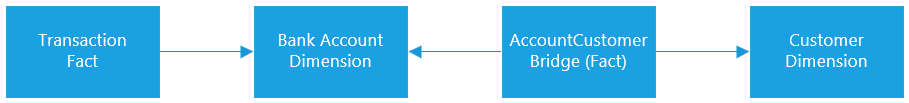
In the example above, a Bank Account has joint Account Holders (Customers). There is no need to derive the Group as it exists as an entity in your source.

Why are Many to Many relationships modeled this way? One reason is that OLAP Cubes recognize this format and faithfully produce the correct aggregations when analyzing the Fact by the Individual Dimension. For example, if you want to sum the Medical Claim amounts for a given Diagnosis, you would select the Diagnosis from the Diagnosis Dimension, drag in your Claim Amount measure, and the OLAP cube would navigate the Bridge and Group relationship to produce the Total Claim Amount for that one Diagnosis.

There is a good tutorial on mssqltips.com that describes setting up this relationship in a Cube.