Persistent Staging

Introduction

This lesson describes Dimodelo Data Warehouse Studio Persistent Staging tables and discusses best practice for using Persistent Staging Tables in a data warehouse implementation. It outlines several different scenarios and recommends the best scenarios for realizing the benefits of Persistent Tables.

What is a Persistent Staging table?

A persistent staging table records the full history of change of a source table or query. The source could a source table, a source query, or another staging, view or materialized view in a Dimodelo Data Warehouse Studio (DA) project. In a persistent table, there are multiple versions of each row in the source. Each version of the row has an effective date and end date marking the date range of when that row version was valid (or in existence).

Technically speaking a persistent table is a bi-temporal table. A bi-temporal table permit queries over two timelines: valid time and transaction time. Valid time is the time when a row is effective. Transaction time denotes the time when the row version was recorded in the database. The persistent table supports transaction time by tagging each row version with an inserted and updated batch execution Id. The batch execution is associated with a start date-time in the batch database. Note that the DA version of the bi-temporal table goes one step further by identifying a last updated transaction date time.

A persistent table exists with other persistent tables in a persistent layer. Unlike a Data Warehouse or Data Vault layer, a persistent layer is only lightly modelled, with its primary purpose being to support the higher layers. In truth, you can model this layer as much or as little as you like. It doesn’t need to be 3rd normal form, again its purpose is to serve higher layers. It would be rare that a persistent layer was queried directly for reporting, but there are some use cases where it makes sense.

Why use a Persistent Layer?

Including a persistent layer in your architecture is a paradigm shift in how you see the data warehouse. In the popular Kimball methodology, without the persistent layer, the data warehouse layer was responsible for persistence. This was problematic, because it only recorded some history, for some entities and for some attributes that were the subject of reporting at the time. If later, the history of another attribute was required, that history simply wasn’t available. In addition, if the logic used to calculate an attribute or measure was wrong, then the source data to recalculate that attribute/measure was no longer available. A persistent layer gives you the flexibility to completely drop and rebuild your data warehouse layer with full history at any time, or just rebuild one dimension or fact. Your data warehouse becomes a true ‘presentation layer’ that can adapt without fear of data loss.

Another key element of a persistent layer is performance. There are two (in my opinion) base strategies for improving ETL/ELT throughput. One is only process changed data (i.e. the delta change set), and the other is parallelism. Because a persistent layer is able to identify what changed and when it is possible to identify the changed set of data. Therefore, all higher layer (e.g. Data Warehouse layer) can be incrementally updated from just the changed set of data. For example, a persistent table may have 500M rows, but on a daily basis, the change set might be just 250k rows. This has a big impact on overall performance.

Other benefits include:

Being able to answer, “why has my report changed”? Types of questions. Often the answer to that is “the source data has changed”. A persistent layer gives you evidence it changed.
It provides for accurate Time-based insight like Churn. For example, in Aged Care, on average how often is the visit schedule changing in the 3 days preceding a home care visit.
Improves data governance. Only with a bi-temporal database can organizations maintain a complete and accurate picture of the past to understand exactly who knew what and did what, when.
Auditing. Supporting Sarbanes-Oxley Compliance and other jurisdiction legislative requirements for audit and accuracy purposes.

Benefits

Provides the ability (or at least the possibility) to re-load with full history if required (due to a change in logic, model or mistakes).
Improves ETL efficiency. It becomes possible to do incremental (delta) loads at all levels.
Without Persistent Tables, it was difficult to do complex transform logic over the data from incremental extracts into staging tables. These staging tables would, on any given day, only have a small subset of rows from the source table/query. It was impossible to join these tables to other tables to get some other representation of the data that needed more than just the subset that was available.
Provides traceability and audit of data.

Persistent Table Details

Persistent table Attributes and Management Columns

Every persistent table contains the following attributes:

HashKey. This is a Hash representation of the of the row used for comparison purposes.
Inserted_Batch_Execution_Id. Dimodelo assigns a new batch execution Id to every execution of the batch. The Inserted_Batch_Execution_Id is the Id of the batch execution that inserted the row.
Updated_Batch_Execution_Id. The last batch execution Id that updated the row.
Row_Effective_Date. The start date and time (to the micro second) that the row version becomes effective. For the first row version this is low date (i.e. 0001-01-01…)
Row_End_Date. The end date and time (to the micro second) that the row version becomes no longer effective. This is always the effective date of the next row version in the series of row versions. Therefore, row effective date and end dates of row versions are contiguous. For the last row version this is high date (9999-12-31….). Joining across row end and effective dates can’t be done with BETWEEN instead use (X >= S2.Row_Effective_Date and X < Row_End_Date)
Row_Is_Latest. 1 indicates the row version is the latest row version.
Row_Is_Deleted. Indicates the row with the same business key has been deleted in the source.
Row_Is_Intra_Batch_Change. Indicates a row version with the same business key appear more than once within the same batch. I.e. the row has been updated multiple times since the last batch run and the source system has provided a row for each update. This indicator is used to trigger a row reordering process for the business key, to get the row versions into the correct order in the persistent table. This indicator must be set by the extract process.
Row_Is_Duplicate. The persistent transform process marks a new row version as a duplicate if it has the same business key and effective date of an existing row version. Duplicates are eliminated from Dimension and Fact transforms.
Row_Is_Late_Arriving. The persistent transform process marks a new row version as a late arriving if its effective date is before the effective date of the current latest row version in the persistent table. This indicator is used to trigger a row reordering process for the business key, to get the row versions into the correct order in the persistent table.

Persist ETL Pattern Overview

The persistent pattern is physically implemented as a stored procedure. There is one persistent stored procedure generated for each extract on a Persistent Tables table in Dimodelo Data Warehouse Studio.

The Persistent pattern relies on the extract process. The extract process extracts data from a source table/file or query and writes the data to a temp table in the staging database.

In the case of a “Full Extract” pattern all the rows are extracted from the source and inserted into the temp table. The rows are then compared to the rows in the persistent table to identify, inserts, updates and deletes, and define the changed data set. The change data set replaces the data in the temp table.
In the case of the “Change tracking” and “Incremental” extracts, only the changed data set is extracted to begin with.

The extract sets the following management columns on the temp table:

Effective date. The effective date of the new/changed/deleted row.
Row Is Deleted. Set to 1 if the row has been deleted. Used by the persistent table in its delete processing.
Reject Indicator. Set to 1 if the mapped expression evaluates to 1. This can be used to eliminate invalid rows from the persistent table.
Segment Num. A number assigned to each row. The first 1M rows = 1, the 2nd 1M rows = 2 etc. The persistent pattern processes 1M row batches. It does this to avoid blowing out the transaction log. It uses the segment num to identify each batch.

The management columns other than segment number are configurable by the user. For example, you could set the effective date to a date in the source (e.g. transaction date). Also, if the source supports soft deletes, you could set the Row Is Deleted indicator via an SQL expression.

Once the extract is complete the persist pattern takes the changed data set in the temp table as its source and “applies” it to the persistent table. It assimilates the changes into the persistent table. See the data flow diagram below:

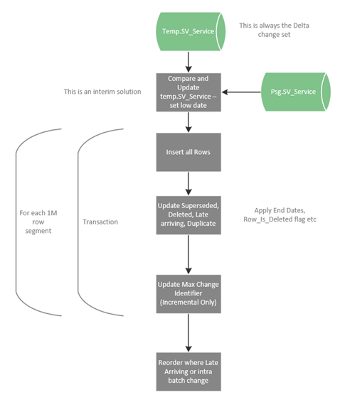
The first step is to join the change set in the temporary table to the persistent table to determine if this is an Insert or Update condition. This is only an interim solution.
The updates are broken into 1M row transactions called segments.
For each segment:
- Start Transaction
  - Insert all rows in the segment.
  - Update (end date) superseded row versions, along with deleted indicator, late-arriving indicator, intra batch change indicator and duplicate indicator.
  - For the incremental pattern, update the max change identifier to the maximum key found in the segment. This ensures that, if a failure occurs, the process restarts from the last committed segment.
- Commit transaction.
End For each Segment
Reorder any rows where an intra batch change or late arriving row has been flagged. For example, if a late arriving row version is flagged then update all rows with the same business key, reordering those rows if necessary, by updating their end date, to get them into the correct order in the series of row versions.

Using Persistent Staging tables at the Dimensional Layer

Persistent Staging tables are technically Bi-Temporal tables. This means they keep all history of change for the source by saving multiple versions of each row in the source. Each version is tagged with an effective and end date. In order to join across multiple persistent staging tables and faithfully reproduce the combined history of those tables, it is necessary to modify the join clause between those tables.

The addition of the below AND clause to the JOIN ON clause in the Transform editor of Dimensions and Facts will correctly join across the tables by effective dates generating a full historical (temporal) result.

The addition of AND (S1.Row_Effective_Date < S2.Row_End_Date and S1.Row_End_Date >= S2.Row_Effective_Date ) makes the query join staging tables S1 and S2 correctly across the effective date ranges of the tables. S1 is staging table 1 (The primary staging table) and S2 is a secondary staging table in the order they appear in the dialog (i.e. S2, S3, S4…)

When specifying the secondary staging table JOIN condition in the Transform editor of Dimensions and Facts, it is necessary to add the above AND clause.

Alternatively, if you are only interested in the latest state of each persistent staging table you can add:

AND S1.Row_Is_Latest = 1 AND S2.Row_Is_Latest = 1

This will mean that the Dimension will be populated from the latest version of each of the staging tables at the time the ETL is run. Join like this negates the ability to reload history for a Dimension.

Restart, Recovery and Monitoring

Restart and recovery are largely reliant on the restart and recovery process of the extract that accompanies the persistent processing. It relies on the extract process to present it the correct changed data set. It faithfully assimilates those changes into the persistent table, regardless of whether they are duplicates of previously presented rows. The persistent table rows are somewhat immutable (other than management columns), so new versions of rows are added when a duplicate is presented.

With the incremental pattern, as each segment is processed, the max change identifier is saved to the zmd.ControlParameters table as part of the transaction. In a restart scenario, the Extract is run, but only extract data for segments that have not already been committed to the Persistent Tables table.

With the Full Extract Pattern, a full comparison between the temporary extract table and the persistent staging table takes place, so only data that has not previously been committed to the persistent staging table is assimilated.

The Persistent pattern writes progress information to the Batch database, TaskProgress table. It writes 1 row per segment it processes. It records start and end times, duration and row insert/update count information, as well as how many rows are deleted and reorganized due to the late arriving scenario.

Every stored procedure execution is recorded in the Task_Execution table along with its start datetime, end datetime, status (in progress, complete, failed) and error information on failure.

Best Practice for Persistent Tables

The next section discusses various Persistent Tables scenarios. An initial investigation of many different scenarios was under taken. The table below shows the recommended approaches. A combination of 1,2 and 3 for the staging layer is preferred, paired with Scenario 5 for the transformation into the dimensional layer.

Scenario 1,2,3 + 5 Overview

The following diagrams depict the various ways to use persistent tables. In the diagrams below,

Scenario 1.

Simple Delta Staging

Scenario 2.

Simple Full Staging

Scenario 3.

Staging from a Query against a source

Scenario 5.

Simple joins at the dimensional model layer

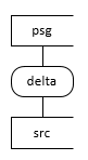
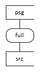
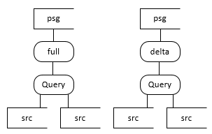
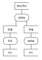
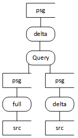
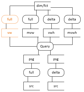
psg = persistent table. src = source table. Query = An SQL query on source tables. Delta = incremental extract (i.e. just the changed data). Full = full extract of all data.

Scenario 1

Scenario 1 represents a data flow directly from a source table (no query) to Persistent Tables (conceptually but not physically skipping staging layer), where only the changed data is extracted. This is the most efficient form of extract. The delta extract is preferred over a full extract from a performance perspective.

Note, the incremental extract pattern doesn’t capture hard deletes, so is not appropriate for source tables where data is hard deleted unless you do periodic full extracts. The change tracking pattern does support hard deletes but is only available for SQL Server tables.

Scenario 2

Scenario 2 represents a data flow directly from a source table (no query) to Persistent Tables (conceptually but not physically skipping staging layer), where all data in the source table is extracted. It is appropriate if the source doesn’t have a change identifier column (e.g. modified date), there is a change identifier column but it’s not reliable, the source table doesn’t have change tracking enabled (SQL Server only) or it is common for the source table to have hard deletes. In this scenario, all data is extracted, and Dimodelo does its own change data capture process to determine the inserts, updates and deletes in the delta change set.

Scenario 3

If the developer can be confident that the logic implemented in the query is either simple enough or static enough that it won’t change, it is appropriate to join source tables in a query as the source of a Persistent Tables table. There is a risk that if the logic changes, the ability to reload history would be lost. It is up to the developer to make that decision. A developer would do this, so he/she could implement the simple left join/where syntax available in scenario 5, and therefore benefit from the full reload with history functionality at the Dimensional layer.

Scenario 5

Scenario 5 applies to the Facts and Dimensions that use Persistent tables as their source. Using this scenario, Dimodelo will generate the temporal joins and effective date resolution automatically, hiding this complexity from the developer. See the Temporal Joins section for a discussion on the complexity of temporal joins. The combination of 1,2, or 3 as sources, and 5 as the transformation into the dimensional layer will currently support full re-load with history in a single batch run.

Dealing with Complex Transformation Logic

If the transformation logic required is more complex than can be supported by the 1,2,3 + 5 scenarios, then the following scenarios are recommended. However, first, consider how you might refactor your code to use scenarios 1,2,3 + 5.

Use either scenario 6 or 7 (vw) depending on the complexity of the kind of query you are willing to write. Don’t write the query to support a historical load.

If, later, historical re-load is required, only then re-factor to include the necessary complex code to enable re-load. Potentially Dimodelo has developed by that stage to be able to inject the necessary temporal resolution code required.

Scenario 6

Scenario 6 can be used to implement complex transformation logic (i.e. Allocations, Aggregation etc). The downside of this approach is that, if the logic contained in the transformation query is wrong, there is no way to reload the data with full history into the derived persistent table.

Scenario 6 with the ‘latest’ query (below) is the preferred option if 1,2,3 + 5 doesn’t work. It materializes the result of the query and can support delta processing. It supports re-load at a higher layer above the derived psg table.

In this scenario, re-load from the raw Persistent Tables table layer is not currently supported. However, given that all data is persistent staged first, the possibility for full reload still exists in a later version of Dimodelo. Dimodelo will support re-load with full history in this scenario in the future. This pattern can also be implemented with Full extract pattern.

The Latest query (below) returns the latest version of each row across the join of source tables. This query won’t support full re-load of the target Persistent Tables table or transform, or any higher layers.

Select *

FROM S1 LEFT JOIN S2

ON S1.key = S2.Key

AND S1.Row_Is_Latest = 1

AND S2.Row_Is_Latest = 1

— Add this for delta processing (i.e. the Incremental Extract pattern)

AND (S1.Inserted_Batch_Id > @Batch_Id OR S2 .Inserted_Batch_Id > @Batch_Id)

If the extract uses the Incremental (delta) pattern, then Inserted_Batch_Id > @Batch_Id is necessary to just extract the rows that have changed.
If the extract uses the Full pattern, then Inserted_Batch_Id > @Batch_Id should not be included.
Note also, it’s more likely that this is implemented as a LEFT JOIN rather than a JOIN. A JOIN will eliminate records in S1 where there is no match in S2.

Scenario 7 (vw)

If you don’t want to materialize the result of the query, then the view option of scenario 7 is best. It doesn’t support re-load with full history, but because all data is persistent staged first, the possibility for that still exists in a later version of Dimodelo.

In this scenario, the query is similar to ‘Latest’ query in scenario 6, but without the filter on Inserted_Batch_Id.

Note there is also a materialized view option in Dimodelo which writes the result set to a table, rather than a virtual view, where the query runs at ETL runtime. The materialized view can perform better if the view is joined to other views in higher layers, or the view is used many times in higher layers. The materialized views supports the write once, read many times concept.